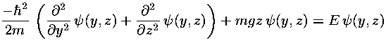
Proceeding exactly as before we have the dimensionless form
We seek to solve this partial differential equation to find
 as a function of y and z.
*=
||2 (* means complex conjugate)
is the probability density, that is the probability of finding the particle
in the (small) interval: [z, z+dz]
is P dz. Since the total
probability must add up to one, proper wavefunctions must satisfy a normalization
condition. In the 1d fall case (where possible particle positions
are restricted to z>0) we had:
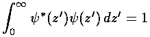 .
.
Probability density is really no more complicated than other
densities you've encountered in physics. To find the mass density
of a small bit of material you divide the mass (dm) of the
little bit of material by the volume (dV) of the
material. The mass density of an object (like you) can then
depend on position (your bones are denser than your flesh).
Similarly in E&M you encountered the idea
of charge density: the charge in some (small) volume
is dQ= dV, naturally the units of
are C/m3, and the total charge
in a volume is found by adding up the bits:
dV, naturally the units of
are C/m3, and the total charge
in a volume is found by adding up the bits:
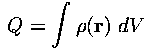 .
.
If we are using Cartesian coordinates the volume element is:
dV=dx dy dz , whereas if we are
using spherical coordinate the volume element is:
dV=r2dr sin d d
d d
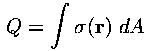
We use a different symbol  to describe the surface charge density. The charge on some
(small) bit of area is dQ=dA,
the units of
are C/m2, and the total charge
in a surface is found by adding up the bits:
to describe the surface charge density. The charge on some
(small) bit of area is dQ=dA,
the units of
are C/m2, and the total charge
in a surface is found by adding up the bits:
 .
.
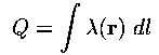
We use yet another symbol (often  )
to describe the linear charge density. The charge on some
(small) bit of a line is dQ=dl,
the units of
are C/m, and the total charge
on a curve is found by adding up the bits:
)
to describe the linear charge density. The charge on some
(small) bit of a line is dQ=dl,
the units of
are C/m, and the total charge
on a curve is found by adding up the bits:
 .
.
In QM we have linear probability densities (as described above
for the 1d fall),
surface probability densities (as in the 2d fall: the probability
of finding the particle in a small dy dz square),
and volume probability density, but we use the same notation
to describe it: *.
Since the above densities have different units, the units of
(unlike most any other symbol in physics)
differ according to the dimensionality of the problem. Accordingly
the normalization condition (that the total probability adds up
to one) will vary with the dimensionality of
the problem:
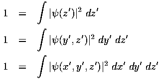 .
.
I have said that classically, motion in the z direction is independent of motion in the y direction. Thus it is natural to assume that the probability density factors:
P(y,z) = Py(y) × Pz(z)
This can be achieved if the wavefunction factors:
(y,z) =
Y(y) × Z(z)
This assumption of separation of variables is unusual in the sense that most functions of two variables cannot be so written as a product of two functions. Therefore the solutions generated by the assumption of separation of variables are a rather restricted class of solutions. Nevertheless, the assumption of separation of variables is usual in the sense that it is the primary approach to finding analytical solutions to partial differential equations. You should find this a bit worrisome: the typical approach to partial differential equations produces only atypical solutions.
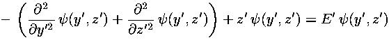
The above total Hamiltonian can be written as the sum of Hamiltonians (one just in y' the other just in z'). The z' Hamiltonian is exactly that solved in the 1d fall case; the y' Hamiltonian is even simpler: there is no potential term --- the motion is "free".
Since the Hamiltonian is the sum of two terms with totally separate variables, we try a product wavefunction:
=Y(y')·Z(z')
As usual with separation of variables, the Schrödinger's equation separates into two terms, one only in y' the other only in z':
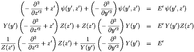
Thus a function just of z' (the first term) plus a function just of y' (the second term) must add to a constant (independent of either z' or y'). This means that each of the two terms must be constant. (For example, if you take the partial derivative of the above equation w.r.t. z', everything is clearly zero except the derivative of the first term. You must conclude that the derivative of the first term is also zero, i.e., it does not depend on z', and hence it must be a constant, which we'll call Ez.) Thus we find separated differential equations for y' and z':
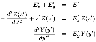
The z' differential equation is exactly as in the 1d fall with Airy functions as solutions. The y' differential equation should be quite familiar to you with sinusoidal solutions like sin(ky') or exp(i ky') where Ey=k2.