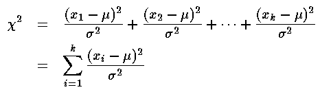
 as:
as:
where the measurements:
{x1, x2, ..., xk}
are supposed to be "normally"
distributed with mean µ and standard deviation  .
.
In the context of an x-y fit, the data are the yi measurements which are assumed to be normally distributed with mean f (xi) and a standard deviation (perhaps different for each point) that depends on the measurement errors:
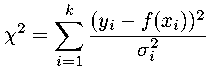
Roughly speaking we expect the measurements to frequently deviate from the mean
by the standard deviation, so:
|(yi-f (xi))| is about
the same thing as . Thus in calculating chi-square
k numbers, each near 1, are being added, so
we expect to approximately
equal k, the number of data points. The "best" fit
will be the one which minimizes these weighted
deviations. Thus,
in the fitting process used here the parameters of the model function
f (x) are adjusted until the minimum value of
is achieved.
That is we think of as a function
of the parameters A and B (and perhaps
C) that occur in the model function. The "best fit"
values of A and B are those at which
is a minimum.
In a simple case, the model function is a line:
f (x) = A + B x
and does not depend on
a or b (i.e., no x-errors). Thus,
if we expand out the terms in the
definition:
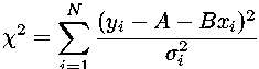
and then bring together terms with the same powers of A and B, we find a simple quadratic form in A and B:
= a A2 + b AB +
c B2 + d A + e B + f
from which one can quickly derive the formula for the location (A,B) of the minimum. (The terms a...f are constants determined by the data.)
Note: In the above case, there is no need to "search" for
the minimum; a bit of algebra
(or calculus) gives the formula for the minimum's location.
The situation with x-errors is more complicated because
then depends on B, so
is no longer a polynomial.
Thus, when
both x and y-errors are present,
a trial-and-error search for the minimum is required. In situations where
the relationship between x and y is well disguised
by large errors, it is possible for that search for the minimum to fail.
As stated above,
we expect to approximately
equal N, the number of data points. If chi-square is
"a lot" bigger than that, the deviations between the data and
the model function must often be more than ;
the fitted curve is not going between the error bars.
If chi-square is
"a lot" smaller than that, the deviations between the data and
the model function must often be less than ;
the fitted curve is going nearly dead center through the error bars.
Both are unlikely situations!
It is convenient to define a reduced χ2
that is the above divided by
N (so reduced
χ2 will have an expected
value of one). (N.B.: We are neglecting here the difference between
the "degrees of freedom" and the number of data points---WAPP
in fact uses "degrees of freedom" in calculating reduced chi-square.)
The below plot shows the likely distribution (pdf technically speaking) of
reduced χ2 for N=10 (red) and
N=100 (blue) [which spans the likely range for
WAPP application]. As you can see, reduced χ2
is likely to be near 1, and becomes increasingly concentrated
about 1 as N increases.
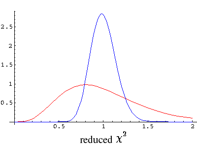
Repeating, the likely situation is to miss each datapoint by
about an error bar (i.e., ), which produces
a reduced χ2 near one.
Hitting each error bar nearly dead center
(producing reduced χ2 < 1)
or missing each
error bar by a lot
(producing reduced χ2 > 1)
are both unlikely situations -- either is "smoking gun"
evidence of a problem with the
experiment. You should always check that your
reduced χ2 is "near" one;
The fit, and most certainly the reported parameter errors,
are some sort of nonsense if
reduced χ2 is not "near" one.
The likelyhood of the fit could be quantified (as it is on most of my pages) as a P value. This is not done here because of the extraordinary sensitivity of P to commonly occurring situations. For example, with N=100, a 10% underestimate of errors can turn a P>.05 fit (at reduced χ2=1.24) into P<.001 (at reduced χ2=1.5). In real experiments errors are rarely known to ±10% accuracy! Additionally, "outliers" (data points whose extraordinary deviation from typical suggests a non-normal error distribution) undermine the validity of a P calculation (since that calculation assumes normally distributed errors). Numerical Recipes, for example, says:
It is not uncommon to deem acceptable on equal terms any model with, say, P>0.001...However, if day-in and day-out you find yourself accepting models with P~10-3, you really should track down the cause.
Errors in "good" experiments may be uncertain by ±50%; errors in introductory labs may be uncertain by a factor of 2. How can much meaning can be attached to the resulting value of χ2? I think the best answer is that the found value of χ2 can act as a goad to better understand the experiment's uncertainties. However, an enticing but dangerous option is to give up on independently determining the errors and instead use the found value of χ2 to determine the errors. Numerical Recipes, for example, says:
In dire circumstances, you might try scaling all your ... errors by a constant factor until the probability becomes acceptable (0.5, say), to get more plausible values for [parameter errors]Unfortunately, in introductory labs, the "goad to better understand" errors can be replaced by the mindless game of repeatedly guessing the reported error until a "good" result is achieved.
In fact the analysis programs we use here in introductory labs (and the non-plus version of WAPP) always re-scales errors before estimating parameter errors. WAPP+ only scales errors in extraordinary circumstances (reduced χ2<0.25 or reduced χ2>4) and it always gives warning when this rescaling has been applied.