Mathematica Assignment

Due February 9, 2005

1 Introduction

Anyone who cannot cope with mathematics is not fully human. At best he is a tolerable subhuman who has learned to wear shoes, bathe and not make messes in the house.

Time Enough for Love
Robert Heinlein

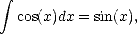
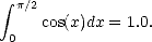
Computational tools beyond handled calculators are now a necessary part of any physicists repertoire. There are a wide variety of available tools including computer codes that are written to solve specific problems, mainstream software tools (such as spreadsheets and databases) which can be applied to physics problems and finally mathematical tools (such as Mathematica, Matlab, Maple, Mathcad, et cetera). We will make use of tools of all of these types in this course. The purpose of this exercise is to introduce you to one of these mathematical tools, Mathematica. Mathematica distinguishes itself from its competitors with its abilities to do exact symbolic, as well as numerical, calculations. These abilities allow Mathematica to, for example, give the solution of

integral cos(x)dx = sin(x),

while most other programs would only be able to solve problems such as i

integral p/2 cos(x)dx = 1.0. 0

In this exercise, you will first work through a Mathematica tutorial to get an idea of Mathematics’s abilities. Then you will use Mathematica to work a more complicated physics problems.

2 Tutorial

Start up Mathematica and open up the “Ten Minute Tutorial.” Carefully work through this tutorial - it should take you much longer than 10 minutes. (Note that you shouldn’t have NumLock activated while using Mathematica.) As you are working through the tutorial feel free to change things in the examples. Try out different numbers, functions, et cetera so that you have a better idea of how Mathematica works. Save a copy of the the tutorial in your home directory so that you can keep track of the changes you make while working through the tutorial.

Complete the following exercises based on the tutorial. Where appropriate print out plots and segments of Mathematica code showing your answers and tape them into your lab notebooks. Also answer the questions in your lab notebook.

On page 3 of the tutorial, calculate 21 to the 31 power and 21. to the 31 power. What is the difference between these results? Why are they different? Which answer would most other mathematical tools give? Why?
On page 5, get an numerical expression for the first 40 digits of e.
On page 6, expand and simplify (a + b)(a - c)(b - d) + (d - c)(b - a)(c + a).
On page 8, plot sinx, sinhx, and sin(sinh(x)) from 0 to 5 on the same plot. Also plot in three dimensions the function arctanxlny over the range from 0 to 5 for x and over the range from -1 to 1 for y.
On page 9, calculate $d ---arcsinh(ax)arcsinh(bx). dx$ The compute $integral arctan(ax).$ Integrate the result. Finally, numerically integrate $integral oo -2x2 e . - oo$
On page 11, solve the system of equations x² - y² = a and x + 3y = b.
On page 13, solve and plot the solution to the differential equation $2 d-y + y+ 10 = 0, dx2$ where y(0) = 0 and y'(0) = 0.

3 Nonlinear Pendulum

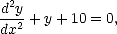
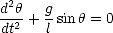
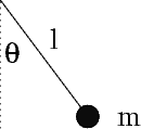
In deriving the motion of a simple pendulum (as seen on the right), using torques (or forces) leads to the equation of motion:

d2h g dt2 +-l sin h = 0

(1)

In order to get this equation in the form of the simple harmonic oscillator equation, we typically assume that the angle is small so that sin , which results in:

d2h g dt2 + lh = 0

(2)

In this exercise you will explore how justified this approximation is. In some parts of this exercise you may have to force Mathematica to make more precise calculations. You may have to use the Accuracy, WorkingPrecision, AccuracyGoal, and PrecisionGoal statements to get useful results.

Find how varying the starting angle alters the angular frequency of the pendulum when you don’t make the small angle approximation. Plot the pendulum frequency versus pendulum (angle) amplitude for amplitudes from 0 to /2 radians. Also, on the same figure include a plot of what the angular frequency versus amplitude is assuming the pendulum is a simple harmonic oscillator. Take enough points so that you get a fairly smooth curve. You don’t have to use Mathematica to plot your results -- any plotting program is fine.
Calculate at what amplitude the angular frequency differs from the ideal angular frequency by 10 % ? By 1 % ? By 0.01 % ? By 0.0001 % ? What does this tell you about the accuracy of the small angle approximation? Under what conditions is this approximation valid?
One of the applications of pendula is in clocks. Calculate how long it would take for a clock using this pendulum to be displaying a time that is off by a minute if the amplitude of the pendulum is 0.1o? 1o? 10o? 30o? 90o?