The Franck–Hertz Experiment
I think it is safe to say that no one understands quantum mechanics. Do not keep saying to
yourself, if you can possibly avoid it, “But how can it be like that?” because you will go “down the
drain” into a blind alley from which nobody has yet escaped. Nobody knows how it can be like
that.
Richard Feynman
1 Introduction
The discreteness of atomic energy levels was first shown directly in the Franck–Hertz experiment
[McGervey, 1983, or almost any modern physics textbook]. The experiment works by colliding electrons with
a gas in a tube. While the original experiment used mercury gas, the version that we will be doing uses neon
gas instead.
In this experiment electrons are emitted from a cathode and then accelerated through the tube by a
potential, U2 . After being accelerated, the electrons are slowed by a potential drop in the opposite direction,
U3 . Then the electrons are collected at the far end of the tube and the current is measured. In a
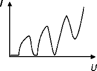
vacuum tube that contains no gas the current would rise steadily as the accelerating voltage, U2, is
increased. The presence of the gas changes this behavior because of collisions of the electrons
with the gas atoms. At first the current does rise with the potential, but when the electrons get
enough energy they inelastically collide with the gas atoms and excite higher energy levels in
the gas (see Figure 1). After these collisions the electrons will have lower energy and due to
the opposing potential, U3 they will not make it to the end of the tube. This will cause the
current to decrease to a minimum. After this minimum, as the potential increases the current
will again increase until the electrons get enough energy to excite the gas twice. This process
continues with the electrons repeatedly exciting the gas atoms. The potential difference between
either the minima or maxima is equivalent to the energy of the excited level. At first glance it
would seem likely that either the difference the maxima and the minima would be the same
and that either could be used. It turns out that they are not the same, and one of things that
you will do in this lab is determine whether the maxima or the minima give you the correct
results.
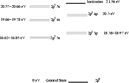
Neon atoms have 10 electrons and a ground state of 1s22s22p6 (see Figure 2). Due to electron spin-related
selection rules, collisions with electrons excite neon atoms from the ground state to the 2p53p
and 2p5 4p states. When falling back toward the ground state by emitting photons the 2p53s
state is also allowed. Recall that you can calculate the wavelength of the photons emitted from
E =  .
.
2 Procedure
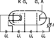
Read through the directions below and set up the circuit as shown in figure 3, but do not turn any of the
power supplies on to begin with. The Franck–Hertz tube is rather fragile and can be broken by
applying incorrect voltages. Have your instructor check your circuit before any power supplies are
switched on. Then work through the directions below again, setting the voltages as suggested,
etc.
- First hook a power supply up across the cathode (UH). This power supply is used to heat the
cathode so that electrons are easily ejected; an AC or DC power would work here. Assuming
that you are using a DC power supply, set this power supply to 5 V. Do not put a large voltage
across the cathode as it could melt the cathode.
- Next, hook a DC power supply from the cathode to the control grid (U1). This potential difference
is used to accelerate the electrons across the tube. It can be raised as high as 5 V, but we will
start with this value at 1 V. You can use a DMM to check the voltage across this portion of the
circuit when you adjust it, but you should not need to continually monitor this voltage.
- A high voltage DC power supply will be needed to accelerate the electrons from the control grid to the
anode grid (U2). The voltage from this supply will be varied throughout the lab. Since the voltage
readings on the power supply itself are not very precise, you should connect a DMM to
measure this potential. To test that your circuit is setup correctly, set this U2 voltage at 70
V. You should be able to see three bands of light between the control and anode grids
in the tube, though it easier to see in the dark. You may want to shade the room lights
from the tube or turn off the lights momentarily. If you do not see any light you may try
increasing U1 by 1 V and then look for the light again. You can repeat this process up to
setting U1 equal to 5 V. If you still do not see the light ask your instructor for assistance.
What color are the bands of light? Once you have seen the light, turn U2 back down to 0
V.
- Now connect the last power supply from the anode to the collector plate (U3). Note that the direction
of this potential difference is opposite that of the other potential drops. The reason for this is
to minimize the current that arrives at the collector grid. Initially set this potential at 5
V.
- Now connect the Pasco electrometer to the BNC connector on the circuit. The electrometer will be used
to (indirectly) measure the current of electrons that arrive at the collector plate. The Pasco electrometer
does not directly measure current, so we will use its voltage measurements (which should be
proportional to the current) as a proxy for the current.
The voltage for the Pasco electrometer can be read directly on the analog scale on the
electrometer, but we will connect it to a PC in order to get more precise measurements.
Start up “Science Workshop” or “Data Studio” on the PC in order to get the readings.
Open up the Franck–Hertz setup from the program in order to view the electrometer’s
measurements.
Note that between each electrometer measurement you will have to hit the zero button on the
electrometer. Failure to do this will lead to spurious results. After hitting the zero button you should
wait at least 5 seconds (and sometimes a minute or more) for the electrometer reading to
stabilize.
Also note that the electrometer voltage readings you get will probably be negative. This is OK, though
in this case you should consider all references to maxima and minima below to refer to the magnitude of
the current.
- Now that the circuit is setup, you should go through the following procedure to adjust the collector
voltage (U3) in order to get the best possible experimental curve. The first step in doing this will be to
roughly find the first minimum greater than 10 V in the current (electrometer voltage) versus voltage
plot for this tube. To do this start with the anode grid voltage (U2) at roughly 10 V. Increase U2 and
take readings of the electrometer voltage versus the anode grid voltage (U2) until you have found the
minimum electrometer voltage between 10 and 30 V. Once you have found the minimum, set the
anode grid voltage back to that reading. Then vary the collector voltage (U3) between 0
and 10 V until you minimize the electrometer voltage. Note that you should consider 0 V
to be the best possible minimum value for the electrometer voltage. Leave the collector
voltage (U3) at the value that minimized the collector voltage throughout the rest of the
experiment.
- Next you should be ready to take the data for the current versus voltage curve. You should take data
for U2 between 0 and 100 V. Do not go any higher than 100 V. While taking the data
concentrate your efforts on determining the maxima and the minima in the curve — the
regions between the maxima and minima are of less interest. You should be able to find 4
minima under 100 V, though the earlier minima may be easier to determine than the later
ones.
3 Data Analysis
- Plot your electrometer voltage versus anode voltage (U2) data. Find the minima and maxima in
U2 and estimate uncertainties for these values.
- Plot the maxima in U2 versus the excitation (maxima) number — 1, 2, 3, .... Find the slope of
this line, which should (assuming that using the maxima is a valid way to do this calculation) be
equal to the excitation energy of neon atoms. Do your results match the expected to within your
uncertainties? Which type of excitations dominate in your plots? What color light was observed?
Is the energy consistent with the color of light that is observed? What energy level transition
would be consistent with the color light that you saw?
- Repeat the same analysis as above for the minima, including answering the questions.
- Analysis of which data, maxima or minima, yields more reasonable energy level transitions?
Explain your answer.
- Do you have any ideas why the maxima or minima give better results?
References
Langley, D., The Franck–Hertz Experiment, 1998.
Leybold Scientific, Franck–Hertz Experiment with Neon, 2003.
McGervey, J. D., Introduction to Modern Physics, Academic Press, Inc., San Diego, California,
1983.