1 Introduction

Though outer space is often described as a vacuum, in actuality there are particles everywhere in the solar system, and there is continuous activity in the region between the celestial bodies. The study of this part of the solar system is called Space Physics [Kivelson et al., 1995], or sometimes Plasma Space Physics after the particles that fill this region. A plasma is a ionized gas, where some of the electrons have been stripped off of atoms creating a mixtures of free electrons and positive nuclei (ions).

Most of the plasma particles filling the solar system can trace their origin to the solar wind, which comes from the outer region of the sun’s atmosphere continually being blown off of the sun. The solar wind typically has a speed of about 400 km/s, though it can range up to about 1200 km/s.

1.1 The Magnetosphere

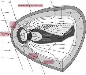
When the solar wind reaches the earth, it interacts with the earth’s magnetic field to form a region known as the magnetosphere (See Figure 1). The earth’s magnetosphere is the region of space where the earth’s magnetic field dominates behavior of the plasma, just as the sun’s magnetic field does in the solar wind. The magnetosphere has many regions, though only a few will be of interest to us in this lab.

The first region of interest (though it is technically part of the magnetosphere) is known as the bow shock. The bow shock is caused by the solar wind meeting an obstruction its flow in the form of the earth. The solar wind has to flow around the the earth, and in doing a shock formed. The bow shock gets its name from the fact that the physics behind the creation of this shock are similar to the shock formed by the bow of a boat as the boat moves through the water.

Nearer to the earth is the magnetopause. The magnetopause marks the furthest that the earth’s magnetic field extends, which makes the magnetopause the boundary of the magnetosphere. The magnetosheath is the region of space between the bow shock and the magnetopause.

1.2 Solar Activity

The surface of the sun, and consequently the solar wind, experiences a variety of events, including flares and coronal mass ejections (CMEs). These events can change both the speed and the number density (particles per volume) of the plasma in the solar wind. When the solar wind from one of these events reaches the earth, the events are called Solar Storms or Magnetic Storms. These variations in the solar wind cause the location of the both the bow shock and the magnetopause vary. Studying the variation in the distance from the earth to the magnetopause is one of the aims of this lab.

The location of the magnetopause is important because the magnetosphere shields the earth and most satellites that go around the earth from the direct effects of the solar wind. When the magnetopause moves, some satellite that are typically protected by the magnetosphere can find themselves in the solar wind. In particular, many satellites are placed in geosynchronous orbits so that they are always above a fixed location on the earth. Geosynchronous orbits are roughly 42000 km (or 6.6 R_E, where 1 R_E equals the radius of the earth) from the center of the earth. During normal solar wind conditions the standoff distance of the magnetopause (the distance from the center of the earth to the point of the magnetopause that is on the line between the magnetopause and the earth) is roughly 10 R_E . During extremely strong Solar Storms the magnetopause can move in closer than geosynchronous orbit. This exposes many satellites to direct contact with extreme solar wind conditions, and satellites are often damaged or lost when this happens.

2 Theory

2.1 Magnetopause Location

The location of the magnetopause along the line between the earth and the sun can be derived by balancing the magnetic pressure of the magnetosphere with the dynamic pressure of the solar wind:

(1)

where r_o is the standoff distance from the earth to the sun in R_E, n_sw is the number density of the plasma in the solar wind in cm^-3, and v_sw is the speed of the solar wind in km/s [Kivelson et al., 1995, pages 173-4]. The entire magnetopause boundary has also been fit to various empirical functions by a number of researchers. We will use expressions from a current set of models for the earth’s magnetopause position for normal solar wind conditions Shue et al. [1997] and extreme eventsShue et al. [1998]. The expressions we will use are

2.2 Coordinate Systems

A variety of different coordinate systems are used to measure locations in space, and in this lab you will have to use data in several of these coordinate systems. More information on these coordinate systems can be found in books [Kivelson et al., 1995] or online [ESA, 2005].

2.2.1 Geocentric Solar Ecliptic

The geocentric solar ecliptic (GSE) coordinate system has its x-axis point from the earth to the sun and its y-axis is in the ecliptic plane (the plane of the earth’s orbit) pointing in the direction of dusk (opposite the direction of the earth’s orbital motion). Its z-axis is in the direction of the ecliptic pole.

2.2.2 Geocentric Solar Magnetospheric

In geocentric solar magnetospheric (GSM) coordinates, as in GSE coordinates, the x-axis points from the earth to the sun. Its z-axis points in the direction of the north magnetic pole. Its y-axis, is perpendicular to the other two, so that a right-handed coordinate system results. The difference between the this system and the GSE system is a simple rotation about the x-axis.

2.2.3 Geocentric Equatorial Inertial

In geocentric equatorial inertial (GEI) coordinates (also known as geocentric solar inertial (GCI)), the x-axis points from the earth to the the first point of Aries (the location of the sun at vernal equinox). This line is where the equatorial and ecliptic planes intersect. The z-axis is parallel to the earth’s rotation axis, and the y-axis complete the the right-handed coordinate system.

3 Simulation

In this portion of the lab you will use a computer simulation to model the location of the magnetopause. The model we will use is called BATS-R-US [Hansen et al., 2002], the Block-Adaptive-Tree-Solarwind-Roe-Upwind-Scheme, which was developed at the University of Michigan. We will be running the simulations on super-computers at NASA-Goddard run by the Community Coordinate Modeling Center (CCMC) [NASA, 2005].

3.1 BATS-R-US Input File

To use BATS-R-US, you must first create an input file which tells the simulation the type of conditions that you would like to simulate. The input file is a simple text file with the conditions at different times listed. A sample input file is available (batrus_input_template.txt) and Table 1 includes a portion of one.

First, note that the first line is a header line which should not be included when you try to run the simulation. Next, note that the first 7 columns of the input file set the time for the conditions that follow. Since we will not be simulating real conditions from a real day, the date we pick is arbitrary, though the usual convention is to pick 1/1/2000 for the date. The time differences are significant, though for our work here we will just use a 5 minute time difference between each of the points that we use. The next six columns give the three components of the solar wind magnetic field in nT, followed by the three components of the solar wind speed in km/s. Note that V_x must be negative, so that the solar wind is moving the earth and that the simulation adds the extra constraint that the magnitude of V_x must be 200 km/s or greater. The final two columns are the solar wind plasma number density in cm^-3 and the solar wind plasma temperature in Kelvin.

In this lab you will complete one simulation run where you vary, in turn, two parameters. In one part of the run you will vary V _x and in the other part you will vary n. For each run you will compare the location of the subsolar point of the magnetopause to the location predicted by equation 1. Ask your instructor what specific range you should use for each. Note that because of the way the simulation interpolates the parameters between input lines that you will always want to have pairs of lines that have the same parameter values. Before submitting your simulation, have your instructor check your input parameters.

3.2 Submitting Your BAT-R-US Simulation Run

As stated explained above, we will be running the BAT-R-US simulation using supercomputers at CCMC. This section describes how to submit your simulation run.

1. Go to http://ccmc.gsfc.nasa.gov/.
2. Click on “Space Weather Models” on left.
3. Under “Global Models: Global MHD” click on the “BATS-R-US” link.
4. Click the “Request a Run” link.
5. Under Runs on Request Submission click the “Submit Request” link.
6. Fill in all required areas and hit the “Submit” button.
7. Under Step 2, choose “BATSRUS: run without RCM” for the simulation.
8. Under Step 3, choose “Simulation with Modeled Conditions” and “Time-Dependent.”
9. Under step 4, et the time at the end of the run equal to the last time in your input file.
10. Leave the dipole tilt at 0 for simplified models.
11. Choose “No Corotation Velocity” and “Semi-Empirical Auroral” and leave the radio flux at 150 since we will not be dealing with the ionosphere, these settings won’t matter.
12. Under Step 5, load the input file. Making sure that you input data looks like the data above with no units at the top. Hit the “Browse” button to find the file. After you have found your file, also input a value for the “Fixed X Component of SW Magnetic Field” — that value will probably be 0. Then hit the “Press” button.
13. Check over the input data to make sure its right. It would also be a good idea to save a copy of the plot that is shown for your records. After you are done, then hit the “Continue” button.
14. Under “Step 6”, set the “Output Frequency” to 300 and press the “Continue” button. Hit “Continue Submission” on the next screen as well.
15. On the “Submit your run” screen, fill in a description of your run in the first text box. In the second text box put in a key word like “educational’. Finally, if you are sure everything is correct, hit the “SUBMIT REQUEST” button.

Once you have submitted the job, you will be sent an email confirmation. After your run is complete, another email will be sent to you.

3.3 Viewing Your Results

After your simulation run has been completed, you can use the online tools to view the results of your run. To get to these tools, hit the “View Simulation Results” link from the CCMC BAT-R-US page. Find your run and click the link. Then click the link to “View Magnetosphere.” This will bring you to a complicated web form which you can use to view your results. The simulation results can be viewed in many different ways, though we will only use a few of them.

3.3.1 Finding Subsolar Magnetopause

First you want want to choose which time point of your simulation to look at under the “Choose data time” option. If you used the data input scheme suggested above where the input parameters are constant for times in a row, then you will want to look at the second time of each pair. In order to find the subsolar point of the magnetopause, it easiest to look at a line plot of various plasma parameters, so choose “Plot Mode” of “Line Plot.” Since the subsolar point in on the x-axis, choose “Y₁”,“Y₂”, “Z₁”, “Z₂” all equal to 0 under the “Choose Plot Area” section at the bottom of the screen. For the x-limits you will want to start out with a range that is sure to include your magnetopause, and then zoom in once you have found the subsolar point of the magnetopause. In order to determine your magnetopause, you should take a look at several of the following data quantities: V _x, B, B_x, B_y, B_z, and n.

The magnetopause boundary should be roughly visible in your plots as the location where the plasma parameters are changing rapidly from the solar wind values which you input, to the magnetosphere values. Recall, though there there are two boundaries near each other in this region. The bow shock, which separates the solar wind from the magnetosheath and the magnetopause which separates the magnetosheath from the magnetosphere. The key point to remember when searching for the magnetopause location, is that the magnetopause defines the outer boundary of the region where the earth’s magnetic field dominates. So while you should be able to tell the location of the magnetopause from some of the other parameters, you should pay the closest attention to the magnetic field components. Come up with your own standard to decide where the magnetopause is and make sure that you use more than one parameter in making your decision. Based on your standard, you should assign a value for the uncertainty of the location of the subsolar point based on how precisely you can determine the locations from your plots. Be sure to save the plots that you use for finding the subsolar point to a file. You should include copies of these plots in your lab notebook.

3.3.2 Making Movie of Results

In order to get a better feel of the global results of your simulation, you should also make a movie of your simulation results. To make this movie you will make plots at a series of times of your simulations results and then combine them to make a simple movie.

To make the movie you will use the same web plotting interface that you used above to make images of your results. You can choose whichever plot type and plasma parameters you would find interesting — experiment with different choices.

Once you have found a plot type you like, make a plot of that type at each time for your simulation. Save a file copy of each plot (by right clicking on the image).

The program mpeg_creator can be used to create a movie from the image files. This is which asks you a few questions and then calls the program mpeg_encode which actually makes the movie. You can access the program from the class web site or from ~jcrumley/public\_html/332/magnetopause/data/mpeg\_creator. To run the program open up a command shell (xterm), change to the directory your data is stored in, and then run the program by typing
~jcrumley/public\_html/332/magnetopause/data/mpeg\_creator
into the command shell. The program will give you instructions as you run it. When you hand in this lab, you should email one copy of your movie to your instructor.

3.4 Questions

1. The distance from the earth to is magnetopause is given roughly by the equation 1. This equation makes the assumption that the solar wind for a typical momentum flux of 2.6 nPa (nv²) leads to a magnetopause location at about 10R_E [Kivelson et al., 1995, page 171]. This is only a general prediction of the location of the magnetopause. From your modeling the solar wind find your empirical constant factor (107.4) for your modeled solar wind. To do this you will need to fit your data to equation 1. Your fit should give you a new value to replace 107.4.
2. What are some possible reasons why in the BATRUS model the value for the magnetopause constant (107.4) changes? What approximations are being made when dealing with MHD in space?

4 Spacecraft Data

For this part of the lab, you will be examining what spacecraft observations of the magnetosphere tell us about about the behavior of the magnetopause under extreme solar wind conditions and how those results compare to the magnetopause models already mentioned. You will use solar wind data to predict where the magnetopause is in the vicinity of a number of satellites and you will check to see if the data from those spacecraft show the spacecraft crossing the magnetopause at the predicted times.

Three specific extreme solar wind events will be examined: October 31 2003, July 15 2000 (Bastille Day storm), and May 4, 1998. For each event the solar wind data was collected from the Advanced Composition Explorer (ACE) satellite from ccmc.gsfc.nasa.gov. ACE resides at about 210 R_E from the earth on the line between the earth and the sun. On board ACE is an array of instruments to measure the solar wind. Solar wind plasma data (SWEPAM) and magnetic field data (MAG) are the two instruments that we will be using data from. The SWEPAM instrument takes the solar wind velocity, ion density, and ion temperature, while MAG takes the magnetic field intensity.

Along with ACE data, we will be using data from several other satellites. These satellites are of several different classes. The GOES satellites are weather satellites and the data that they take that is of interest to us is magnetic field data (MAG) and energetic particle data (EP). The L satellites are run by Los Alamos National lab and contain plasma data, low and high energy ions as well as electron number densities. All GOES and L satellites are in geosynchronous orbit. We will also be using data from two NASA satellites with more interesting orbits — Geotail and Polar. Geotail has ion number density and speed data (CPI), and magnetic field data (MGF) that we will be using. Polar has magnetic field (MFE) data that we will be using. During the events listed above these satellites spend at least some time inside the magnetosphere. The point of this lab is to check the satellite data for signs of having crossed the magnetopause and compare that to predictions of equation 2.

4.1 Procedure

For each event the earth’s magnetopause location has already been calculated using equation 2 based on ACE data which is also included in the spreadsheet. The position of the magnetopause along with the location of a particular satellite. These results are included in spreadsheet files which have been stored under the data directory on the course web site. Along with the spreadsheet files are data files which you will want to add to the spreadsheet in order to do further analysis. These files contain either magnetic field data or ion number density data.

1. Magnetic field data contains MAG, MFE, or MFG in the file (G0_K0_MAG_65544.txt) the txt is the actual data and the .gif is a graph of the data.
2. Ion data should be in a MPA (L1_K0_MPA_65778.txt) file from which you want the “low P DENS” info. Or it will be an EP# (G0_K0_EP8_225752.txt) file where a large flux usually means a transfer between barriers.

In the program gnumeric, you can add the data to the spreadsheet by opening it as a file of type “Text Import”. Once you have the data imported, you can plot it and compare it to the plot of the position of the magnetopause. Depending on the data that you are using, it may be easiest to have one plot with the spacecraft data open and another plot showing the spacecraft position as well as the predicted position of the magnetopause. If you have the same time scale on each plot, then you can compare the features on each plot to determine whether the data supports the idea of having magnetopause crossings where they are predicted by the other plot.

Note that you can add legends and axis labels on gnumeric plots. To do so right-click on the plot and open its “Properties” window. To add a legend highlight “Chart1”, click the “Add” button and choose “Legend”. To add axis labels, highlight the axis name that you want to add a label to, click the “Add” button and choose “Label.”

The Geotail data from October 2003 has been done for you so you know what you are looking for and how to interpret the data. Some explanations have been saved on the spreadsheet for the event.

For each satellite there is some sort of data to try and confirm the location of the magnetopause. In some cases the satellite never crosses the theoretical magnetopause, but you need to check that the data shows the same thing. When examining the satellite data, pay particular attention to the times at which the theoretical magnetopause location plot shows the satellite crossing the magnetopause. Note any signs of a magnetopause crossing. Based on your examination of the data and the theoretical magnetopause location, determine if you believe the satellite crossed the magnetopause and if so at what time[s].

Listed below are the events and the data that we have available for them. Your instructor will tell you which events you should look at.

4.2 Questions

1. For which satellite and event pairs did you find magnetopause crossings? How strong do you believe the evidence is for a crossing in this case?
2. In any of your events does it appear that the satellite crossed the magnetopause repeatedly? If so, does it seem as though magnetopause is moving back and forth over the satellite? What could explain this type of behavior?
3. Which data did you find easier to interpret - ion or magnetic field ? Why?
4. Which spacecraft data did you find easier to interpret? Why? Do you think that this is a result of the behavior of a specific event? Or of the satellite’s position during that event?
5. In any of these cases does the data show the magnetopause crossing geosynchronous orbit?

References