|
|
Though outer space is often described as a vacuum, in actuality there are particles everywhere in the solar system, and there is continuous activity in the region between the celestial bodies. The study of this part of the solar system is called Space Physics [Kivelson et al.,
Most of the plasma particles filling the solar system can trace their origin to the solar wind, which comes from the outer region of the sun’s atmosphere continually being blown off of the sun. The solar wind typically has a speed of about 400 km/s, though it can range up to about 1200 km/s.
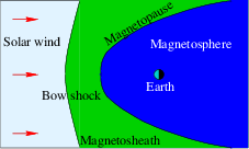
When the solar wind reaches the earth, it interacts with the earth’s magnetic field to form a region known as the magnetosphere (See Figure 1). The earth’s magnetosphere is the region of space where the earth’s magnetic field dominates behavior of the plasma, just as the sun’s magnetic field does in the solar wind. The magnetosphere has many regions, though only a few will be of interest to us in this lab.
The first region of interest (though it is not technically part of the magnetosphere) is known as the bow shock. The bow shock is caused by the solar wind meeting an obstruction its flow in the form of the earth. The solar wind has to flow around the the earth, and in doing a shock formed. The bow shock gets its name from the fact that the physics behind the creation of this shock are similar to the shock formed by the bow of a boat as the boat moves through the water.
Nearer to the earth is the magnetopause. The magnetopause marks the furthest that the earth’s magnetic field extends, which makes the magnetopause the boundary of the magnetosphere. The magnetosheath is the region of space between the bow shock and the magnetopause.
Nearer still to the earth are the ring currents and radiation belts (also known as the Van Allen belts). These areas are located within a few RE of the earth above the equator and low latitudes. The relatively high number of high energy particles in these areas make this region dangerous for spacecraft and difficult to observe.
The surface of the sun, and consequently the solar wind, experiences a variety of events, including flares and coronal mass ejections (CMEs). These events can change both the speed and the number density (particles per volume) of the plasma in the solar wind. When the solar wind from one of these events reaches the earth, the events are called Solar Storms or Magnetic Storms. These variations in the solar wind cause the location of the both the bow shock and the magnetopause vary. Studying the variation in the distance from the earth to the magnetopause is one of the aims of this lab.
The location of the magnetopause is important because the magnetosphere shields the earth and most satellites that go around the earth from the direct effects of the solar wind. When the magnetopause moves, some satellite that are typically protected by the magnetosphere can find themselves in the solar wind. In particular, many satellites are placed in geosynchronous orbits so that they are always above a fixed location on the earth. Geosynchronous orbits are roughly 42000 km (or 6.6 RE, where 1 RE equals the radius of the earth) from the center of the earth. During normal solar wind conditions the standoff distance of the magnetopause (the distance from the center of the earth to the point of the magnetopause that is on the line between the sun and the earth) is roughly 10 RE. During extremely strong Solar Storms the magnetopause can move in closer than geosynchronous orbit. This exposes many satellites to direct contact with extreme solar wind conditions, and satellites are often damaged or lost when this happens.
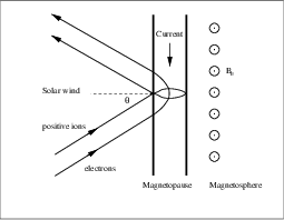
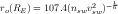
The location of the magnetopause along the line between the earth and the sun can be derived by balancing the magnetic pressure of the magnetosphere with the dynamic pressure of the solar wind (see Figure 2. The equation for this balance takes the form:
 | (1) |
where ro is the standoff distance from the earth to the magnetopause along the line to the sun measured in RE, nsw is the number density of the plasma in the solar wind in cm-3, and vsw is the speed of the solar wind in km/s [Kivelson et al.,
A variety of different coordinate systems are used to measure locations in space, and in this lab you will have to use data in several of these coordinate systems. More information on these coordinate systems can be found in books [Kivelson et al.,
The geocentric solar ecliptic (GSE) coordinate system has its x-axis point from the earth to the sun and its y-axis is in the ecliptic plane (the plane of the earth’s orbit) pointing in the direction of dusk (opposite the direction of the earth’s orbital motion). Its z-axis is in the direction of the ecliptic pole.
In geocentric solar magnetospheric (GSM) coordinates, as in GSE coordinates, the x-axis points from the earth to the sun. Its z-axis points in the direction of the north magnetic pole. Its y-axis, is perpendicular to the other two, so that a right-handed coordinate system results. The difference between the this system and the GSE system is a simple rotation about the x-axis.
In geocentric equatorial inertial (GEI) coordinates (also known as geocentric solar inertial (GCI)), the x-axis points from the earth to the the first point of Aries (the location of the sun at vernal equinox). This line is where the equatorial and ecliptic planes intersect. The z-axis is parallel to the earth’s rotation axis, and the y-axis complete the the right-handed coordinate system.
In this portion of the lab you will use a computer simulation to model the location of the magnetopause. The model we will use is called BATS-R-US [Hansen et al.,
This code is a magnetohydrodynamics (MHD) simulation. In MHD, a plasma is approximated as a quasi-neutral fluid, and that fluid is assumed to be governed by equations that are generalizations of the equations of fluid dynamics. MHD simulations ignore the behavior and physics of individual particles, and deal with the collective behavior of the plasma as a fluid. For this reason, MHD simulations work well on large scales, but miss much of the smaller scale physics.
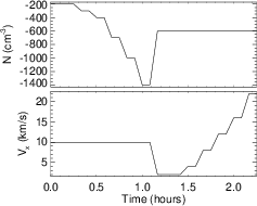
To use BATS-R-US, you must first create an input file which tells the simulation the type of conditions that you would like to simulate. The input file is a simple text file with the conditions at different times listed. A sample input file is available (batrus_input_template.txt) and Table 1 includes a portion of one.
First, note that the first two lines are a header line which should not be included when you try to run the simulation. Next, note that the first 7 columns of the input file set the time for the conditions that follow. Since we will not be simulating real conditions from a real day, the date we pick is arbitrary, though the usual convention is to pick 1/1/2000 for the date. The time differences are significant, though for our work here we will just use a 5 minute time difference between each of the points that we use. The next six columns give the three components of the solar wind magnetic field in nT, followed by the three components of the solar wind speed in km/s. Note that Vx must be negative, so that the solar wind is moving the earth and that the simulation adds the extra constraint that the magnitude of Vx must be 200 km/s or greater. Also note that the components of B must not b 0. The final two columns are the solar wind plasma number density in cm-3 and the solar wind plasma temperature in Kelvin.
|
|
|
In this lab you will complete one simulation run where you vary, in turn, two parameters. In one part of the run you will vary V x and in the other part you will vary n. For each run you will compare the location of the subsolar point of the magnetopause to the location predicted by equation 1. Ask your instructor what specific range you should use for each. Note that because of the way the simulation interpolates the parameters between input lines that you will always want to have consecutive lines that have the same parameter values. If there are places where you have large jumps in input parameters (typically when you go from constant V x to constant n), you should have four lines in a row with the same values in order to give the simulation more time to settle down to an equilibrium For most simulations, there will be two places where you need to do this - at the beginning of the simulation and in the middle. Before submitting your simulation, have your instructor check your input parameters.
Make sure to save your input parameters in your lab notebook. Include either your input txt file or the graph of conditions, or preferably both.
As stated explained above, we will be running the BATS-R-US simulation using supercomputers at CCMC. This section describes how to submit your simulation run.
Once you have submitted the job, you will be sent an email confirmation. After your run is complete, another email will be sent to you.
After your simulation run has been completed, you can use the online tools to view the results of your run. You may get a link directly to your results. Or you can hit the “Simulation Sevices— Visualization” link from the main CCMC page. Then click the “archived” link. Then click “Search the Simulation Result Databse” and scroll down to the “Global Magnetosphere Models Results”. Find your run either by searching for your name or by browsing through the list of results, then click the link. Then click the link to “View Magnetosphere.” This will bring you to a complicated web form which you can use to view your results. The simulation results can be viewed in many different ways, though we will only use a few of them.
First, you should use the web form to make an animated movie of your results. To do this choose “Create GIF movie with current plot settings” near the top of the screen. Then just below that set the start and end time of your movie to the start and end time of your simulation run and add your email address. Then you need to choose the type of plot to use for the movie — for this first movie, just use the default choices of “ColorContour2D” and “N” (number density). Near the bottom, choose a plot range of X=(-80, 25), and Z=(-50, 50). Choose Y to be the cut plane with a value of y=0. Also, Click the “Show magnetic topology” Checkbox. You will probably need to click the “Show advanced options” box.
Then hit the “Update Plot” button and a short time later your will receive a link to your movie.
You should also try an animated gif with plot type “ColorContour (2D)”, “Q 1:” “B”. Click the “Show magnetic topology” and “ Show boundary of closed field lines (magnetopause on dayside) ” checkboxes. Also, change the plot range to Y= (-50, 50) with a Z cut plane at z=0.
Save copies of your movies in your home directories and email copies of them to your instructor (or you can send a link to it online). Print one frame from each movie on a color printer, and include it in your lab notebook. Describe what you see in the movies in your lab notebook.
The simulation can determine the magnetopause location for you. To use these functions, go back to the page where you chose “View Magnetosphere” and now choose “View Magnetopause standoff and closest approach within 30 deg. of Sun-Earth line (local noon).”
For this plot type, choose to plot your whole time range (which will probably be set automatically. Also, choose to display all three data types that are possible on this plot: “mpnose”, “rmin”, and “lt_at_rmin”. Take the uncertainity in all of the upplied distances to be 0.1 RE. The one of these that you will be most interested in is “mpnose” which is the distance from the center of the earth to the subsolar point of the magnetopause. Save a copy of this plot. Also click the option at the bottom to save the data to a text file, and be sure to save the text file.
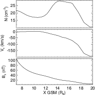
First you want to choose which time point of your simulation to look at under the “Choose data time” option. If you used the data input scheme suggested above where the input parameters are constant for several times in a row, then you will want to look at the last time for each set pf parameters. In order to find the subsolar point of the magnetopause, it easiest to look at a line plot of various plasma parameters, so choose “Plot Mode” of “Line Plot.” Since the subsolar point in on the x-axis, choose “Y1”,“Y2”, “Z1”, “Z2” all equal to 0 under the “Choose Plot Area” section at the bottom of the screen. For the x-limits you will want to start out with a range that is sure to include your magnetopause, and then zoom in once you have found the subsolar point of the magnetopause. In order to determine your magnetopause, you should take a look at several of the following data quantities: V x , B, Bx, By, Bz, and n. Figure 4 is an example of the sort of plot that you will want to make.
|
|
The magnetopause boundary should be roughly visible in your plots as the location where the plasma parameters are changing rapidly from the solar wind values which you input, to the magnetosphere values. Recall, though there there are two boundaries near each other in this region. The bow shock, which separates the solar wind from the magnetosheath and the magnetopause which separates the magnetosheath from the magnetosphere. The key point to remember when searching for the magnetopause location, is that the magnetopause defines the outer boundary of the region where the earth’s magnetic field dominates.
In Figure 4, the magnetopause is located at roughly 11 RE. In the number density plot, the bump in the number density corresponds to the buildup of plasma in the magnetosheath, so the inner boundary of that bump corresponds to the magnetopause. In the plot of the x-component of the velocity, the magnetopause is seen as the location where the value goes to 0, since the plasma from the solar wind is diverted around the magnetosphere at the magnetopause. Finally, in the plot of the z-component of the magnetic field, there is an almost imperceptible shift at 11 RE. So in this case, counter-intuitively, it is easier to find the magnetopause in the plasma results for the the simulation than in the magnetic field results.
Come up with your own standard to decide where the magnetopause is and make sure that you use more than one parameter in making your decision. Note that the point where two lines representing different quantities cross has no physical significance. Based on your standard, you should assign a value for the uncertainty of the location of the subsolar point based on how precisely you can determine the locations from your plots. Be sure to save the plots that you use for finding the subsolar point to a file. You should include copies of these plots in your lab notebook. Note that if you defined your input parameters as suggested, then you only need to find the magnetopause location for the last time for each of the sets of input parameters that have the same parameter values.
The distance from the earth to is magnetopause is given roughly by the equation 1. This equation makes the assumption that the solar wind for a typical momentum flux of 2.6 nPa (nv2) leads to a magnetopause location at about 10RE [Kivelson et al.,1995, p. 171]. This is only a general prediction of the location of the magnetopause. Plot your two sets of estimates of the magnetopause location. From your results find your empirical constant factor (similar 107.4) for both of your sets of estimates of the magnetopause location. To do this you will need to fit your data to equation 1. You should come up with four fits to this equation: one for each section of your input data (constant V and constant n for the solar wind) for each estimate of the magnetopause location [your estimates (Section 3.3.3 and the simulation’s estimates (Section 3.3.2)].
For this part of the lab, you will be examining what spacecraft observations of the magnetosphere tell us about the behavior of the magnetopause under extreme solar wind conditions and how those results compare to the magnetopause models already mentioned. You will use solar wind data to predict where the magnetopause is in the vicinity of a number of satellites and you will check to see if the data from those spacecraft show the spacecraft crossing the magnetopause at the predicted times.
Three specific extreme solar wind events will be examined: October 31 2003, July 15 2000 (Bastille Day storm), and May 4, 1998. For each event the solar wind data was collected from the Advanced Composition Explorer (ACE) satellite from cdaweb.gsfc.nasa.gov. ACE resides at about 210 RE from the earth on the line between the earth and the sun. On board ACE is an array of instruments to measure the solar wind. Solar wind plasma data (SWEPAM) and magnetic field data (MAG) are the two instruments that we will be using data from. The SWEPAM instrument takes the solar wind velocity, ion density, and ion temperature, while MAG takes the magnetic field intensity.
Along with ACE data, we will be using data from several other satellites. These satellites are of several different classes. The GOES satellites are weather satellites and the data that they take that is of interest to us is magnetic field data (MAG) and energetic particle data (EP). The L satellites are run by Los Alamos National lab and contain plasma data, low and high energy ions as well as electron number densities. All GOES and L satellites are in geosynchronous orbit. We will also be using data from two NASA satellites with more interesting orbits — Geotail and Polar. Geotail has ion number density and speed data (CPI), and magnetic field data (MGF) that we will be using. Polar has magnetic field (MFE) data that we will be using. During the events listed above these satellites spend at least some time inside the magnetosphere. The point of this lab is to check the satellite data for signs of having crossed the magnetopause and compare that to predictions of equation ??.
For each event the earth’s magnetopause location has already been calculated using equation ?? based on ACE data which is also included in the spreadsheet. The position of the magnetopause along with the location of a particular satellite. These results are included in spreadsheet files which have been stored under the data directory on the course web site. These spreadsheets can be read using the “gnumeric” program. The predicted magnetopause location and the satellite’s distance from the earth have also been saved into text files ending with “.txt”, but are otherwise named the same as the spreadsheets. You will need to use these text files to create your own plots of the predicted magnetopause crossings. Along with the spreadsheet files are data files which you will want to compare to the magnetopause location data. These files contain either magnetic field data, ion number density data, or particle flux data. The data files that you will want to use all end in “_nt.txt”.
|
|
Figure 5 shows an example of the type of analysis you will be doing with this data, though you do not have to try to get all of the data on one plot. To make your plots, you can use the the iplot feature of a program called idl. Directions on how to use this program are in the file iplot_tutorial.txt.
Depending on the data that you are using, it may be easiest to have one plot with the spacecraft data open and another plot showing the spacecraft position as well as the predicted position of the magnetopause. If you have the same time scale on each plot, then you can compare the features on each plot to determine whether the data supports the idea of having magnetopause crossings where they are predicted by the other plot.
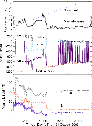
The example data in Figure 5 shows Geotail data from October 31, 2003. On that day a large CME hit Earth, causing auroras that were visible throughout much of the United States.
The top panel of Figure 5 predicts several magnetopause crossings, but the most notable crossings are at roughly 5:00, 10:00, and 11:00. From 1:30–5:00 and from roughly 10:00–11:00, Geotail is predicted to be inside the magnetosphere. In other words, at those times Figure 5 shows the magnetopause further from the Earth than the spacecraft is. For most of the rest of that day Geotail was inside the magnetosphere. The data in the middle and bottom panels of Figure 5 shows the crossing from inside to outside the magnetosphere at 11:00 and the data also shows other magnetopause crossings, though as described below the crossings seen in the data differ a bit from the predictions. Note that the prediction of the magnetopause location is based on solar wind data from outside the magnetosphere. The time its takes the solar wind to get to the spacecraft from the place at which it is measured varies, but it typically about 15 minutes. So we should expect to see magnetopause crossings slightly earlier in the predictions than in the data.
The middle panel of Figure 5, which shows the ion flow velocity measured by Geotail and the x-component of the solar wind speed measured by ACE, has three visible regimes. During this day the x-component of the solar wind velocity slowly changes from -1200 km/s to -800 km/s. From 0:00–5:00 most of the Geotail ion flow velocity data is missing. From 5:00–11:00 the three components of the ion flow velocity measured by Geotail oscillate near values of -700 km/s, -400 km/s, and 200 km/s respectively. While from 11:00–24:00 the y- and z-components oscillate near 0 km/s, and the x-component is based at roughly -1000 km/s, with spikes up to almost 0 km/s. The behavior of the x-component during this last time period can be interpreted as being due to the spacecraft being just outside the magnetopause in the magnetosheath. When the x-component is near -1000 km/s it matches the solar wind speed, suggesting that Geotail is outside the magnetopause at those times. The noisiness of these measurements of the ion speed in the magnetosheath is likely due to reflection of the solar wind ions off the magnetopause and the movement of the magnetopause as the solar wind conditions vary.
The velocity measurements act much differently from 5:00–11:00, suggesting that the spacecraft is inside the magnetosphere during those times. Notice that during this time there are several short time periods where all components of the data have spike which match their magnetosheath values. This suggests that during this time period the spacecraft is near the magnetopause boundary and that fluctuations in the solar wind cause the magnetopause to oscillate back and forth across Geotail’s position.
The third panel, showing Geotail’s magnetic field measurements, has similar regions of behavior. From 0:00–11:00 all three components have spiky measurements which trend downward. The downward trend is due to the decreasing magnitude of the Earth’s dipole field as Geotail gets further from Earth, while the spikes are due to disturbances in the plasma in the magnetosphere during this magnetic storm. From 11:00–24:00, the three components are steadier and oscillate near 10 nT, 5 nT, and -10 nT, respectively. During this time Geotail is in the magnetosheath where the solar wind magnetic field dominates. Note that during several of the spikes in the magnetic field which occur between 0:00 and 11:00, that the magnetic field matches the magnetosheath values. This supports the idea that the magnetopause oscillated back and forth past the spacecraft, as was mentioned with the ion velocity data.
The number density plot shows similar behavior. There is a large spike in the number density just after 5. That peak slowly decays until about 10, after which there are several smaller peaks. Once again, this plot shows Geotail inside the magnetopause from roughly 5-10, and in the magnetosheath afterwards.
For the cases you will look at, for each satellite there is some sort of data you should examine to try to confirm the location of the magnetopause. In some cases the satellite never crosses the theoretical magnetopause, but you need to check that the data shows the same thing. When examining the satellite data, pay particular attention to the times at which the theoretical magnetopause location plot shows the satellite crossing the magnetopause. Note any signs of a magnetopause crossing. Based on your examination of the data and the theoretical magnetopause location, determine if you believe the satellite crossed the magnetopause and if so at what time[s].
***Be sure to analyze potential magnetopause crossings in each set of data before going on to the questions.*** As part of that analysis, you should describe whether each data plot supports any potential crossings that you see in the spacecraft position / predicted magnetopause position plot. It is a good practice to write that analysis on the page you taped made the plot, or on the facing page.
Listed below are the events and the data that we have available for them. Your instructor will tell you which events you should look at.
| Event | May 4, 1998 | July 15, 2000 | October 31, 2003 |
| Satellites | GOES 9 | GOES 8 | Geotail |
| L4 | GOES 10 | GOES 10 | |
| L7 | L1 | GOES 12 | |
| Polar | L4 | L0 | |
| L9 | L1 | ||
| L4 | |||
| L7 | |||
For this experiment (and the others) you should add a conclusion discussing and critiquing the lab and your results.
Simulation results have been provided by the Community Coordinated Modeling Center at Goddard Space Flight Center through their public Runs on Request system. The CCMC is a multi-agency partnership between NASA, AFMC, AFOSR, AFRL, AFWA, NOAA, NSF and ONR. The BATS-R-US Model was developed by Tamas Gombosi et al. at the Center for Space Environment Modeling at the University of Michigan. Spacecraft key parameter data provided by CDAWeb. Solar wind data shown here is from ACE SWEPAM provided by D. J. McComas from SWRI and ACE MFI provided by N. Ness from Bartol Re- search Institute. Data shown here from Geotail MGF provided by S. Kokubun at STE- LAB, Nagoya University, and Geotail CPI pro- vided by L. Frank at University of Iowa. GOES 8, 9,10, and 12 data provided by T. Onsager and H. Singer from NOAA. L1, L4, L7, and L9 data shown here was provided by provided by E. Dors, M. Thomsen, and D. McComas from LANL. GOES 8, 9,10, and 12 data shown here was provided by T. Onsager and H. Singer from NOAA. Polar data shown here was provided by C. Russell (UCLA), D Gurnett (U. Iowa) and W.K. Peterson (LASP/University of Colorado).
ESA, Coordinate systems and transformations, http://www.spenvis.oma.be/spenvis/help/background/coortran/coortran.html , 2005.
Hansen, K., G. Tóth, A. Ridley, and D. DeZeeuw, BATS-R-US User Manual: Code Version 7.5.0, http://csem.engin.umich.edu/docs/HTML/USERMANUAL/USERMANUAL.html, 2002.
Kivelson, A., M. G. Kivelson, and C. T. Russell, Introduction to Space Physics, Cambridge University Press, London, 1995.
NASA, http://ccmc.gsfc.nasa.gov/, 2005.
Shue, J.-H., J. K. Chao, H. C. Fu, C. T. Russell, P. Song, K. K. Khurana, and H. J. Singer, A new functional form to study the solar wind control of the magnetopause size and shape, J. Geophys. Res., 102(a5), 9497–9512, 1997.
Shue, J.-H., et al., Magnetopause location under extreme solar wind conditions, J. Geophys. Res., 103(A8), 17,691–17,700, 1998.