A Severe Strain on the Credulity
As a method of sending a missile to the higher, and even to the highest parts of the earth’s atmospheric envelope, Professor Goddard’s rocket is a practicable and therefore promising device. It is when one considers the multiple-charge rocket as a traveler to the moon that one begins to doubt ... for after the rocket quits our air and really starts on its journey, its flight would be neither accelerated nor maintained by the explosion of the charges it then might have left. Professor Goddard, with his “chair” in Clark College and countenancing of the Smithsonian Institution, does not know the relation of action to re-action, and of the need to have something better than a vacuum against which to react . . . Of course he only seems to lack the knowledge ladled out daily in high schools.
The problem of the flight of a rocket is an interesting problem for both practical and more theoretical reasons. The flight of a rocket can be pursued at several different levels theoretically. The simplest level is a basic constant force problem using Newton’s Laws:
|
| (1) |
At this simple level we would only deal with two forces — gravity and rocket thrust. In the case of vertical flight this leads to:
 | (2) |
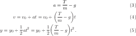
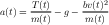
where T is the thrust. Assuming constant thrust, solution of this differential equation is trivial:
This solution is appropriate in cases such as in when the rocket’s mass is almost constant and air resistance is negligible, but neither of these conditions will hold for this lab.In order to analyze our model rockets we will have to deal with at least three complicating factors. In our rocket engines, thrust as a function of time will be much closer parabolic than constant, so we will have to deal with varying the thrust. Next, the mass of the rocket will change as it burns off its propellant, so we will not be able to use a constant mass in our equations. Finally, the air resistance will add another force to our equation of motion.
The simplest time-varying thrust that we can consider is essentially a square wave — the rocket engine is on at some constant value until it burns out. While this is not a good approximation to our rocket, it is a useful case to consider because it shows some features that will also appear in our more realistic thrust curves. The on/off character of this type of thrust curve leads to the technique of splitting the problem in two. First, solve for the rocket’s motion for the case of constant thrust, using the equations 3–5. Then after the rocket engine quits, start with initial conditions based on when the engine stopped and solve using the same equations with a thrust of 0.
In order to deal with thrust curves that are more realistic than square waves, we need to come up with expressions for thrust as a function of time: T → T(t). We will find the thrust curves in two ways: by using the manufacturer’s published curves (Section 2.2) and experimentally using a force meter (Section 2.3).
Since we will not be able to directly measure how the mass of the rocket engine changes during the rocket’s flight, we a need a proxy that will allow us to deal with mass as a function of time (m → m(t)). The obvious choice is to assume that for each unit of mass that is lost a constant amount of thrust is derived:
 | (6) |
or
 | (7) |
where α is a proportionality constant. With this idea we can use the initial (mei) and final (mef ) mass of the rocket engine along with our thrust curve to get me(t). Solving this differential equation we get:
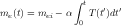 | (8) |
or after the engine is exhausted:
 | (9) |
The quantity ∫ T(t)dt is known as the impulse, and it is provided by the engine manufacturer, though it also can be calculated directly from the thrust function. So we can find α using the equation 9 and then use it in the equation 8 for the time varying mass, me (t).
Air resistance is a complicated subject and for most real problems it cannot be dealt with analytically. Typically one of a variety of approximations is applied depending upon which fluid regime the problem falls under [?]. For this lab we will use :
 | (10) |
where here “-” means that the drag force is in the opposite direction from the direction that the rocket moves and b is the drag constant. Other common forms for the drag force depend on the speed to the first power. The constant b depends on the fluid the rocket is moving through and the shape of the rocket:
 | (11) |
where ρ is the density of air, cd is the drag coefficient, and A is the surface area of the cross-section of the rocket. We will measure the cross-sectional area, and the density of air can be determined from the ideal gas law and the weather conditions at the time of the flight of the rocket. The drag coefficient depends on the shape of the rocket and the smoothness of its surface. The drag coefficient is one of the major unknown quantities that we will determine in this lab. Values for this quantity should end up being somewhere between 0.2 and 2.
Since the form for the drag force law changes as the speed of an object changes, the drag coefficient is not constant over wide speed ranges. In this lab we will first use one type of rocket engine to determine the drag coefficient. With another type of rocket engine we will then use the drag coefficient as a known value, and predict the maximum height of the rocket.
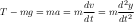
Finally, we get to an equation including time-varying thrust, time-varying mass, and air resistance
 | (12) |
This is the equation that we will solve to find the drag coefficient for the rocket.
Follow the instructions included with the rockets for putting your rocket together. Put you parachute together, but do not attach the nose cone or parachute to the shock. You will attach the cargo section to the shock cord when you are going to launch. Sand and paint your rockets in order to have a smooth surface that minimizes drag.
For manufacturers thrust curves, use the files at http://www.physics.csbsju.edu/~jcrumley/370/rocket/. Take the force uncertainty in these files to be ±0.1 N. Note that for this lab (and for the others), you should keep electronic copies of any plots that you make.
Thrust curves will be determined using a force meter connected to a computer. Make sure that the interface is set to take data at a rate of at least 100 samples per second. See the pictures on the web for one possible way to set up this equipment. The equipment should be setup under a hood to minimize the smoke dispersal through the building. Calibrate the force meter with known masses. Have your instructor check your setup before firing the rocket engines.
The Vernier Force Sensor, LabQuest Mini sensor interface, and Logger Pro software. When you plug connect the LabQuest Mini to the computer its LED will initially be red. If the interface is getting enough power, the LED will turn amber. Then, when you start LoggerPro, it should turn green. If it does not turn green, the sensor will not work. Not that if you are using a USB extension cable, you may also need to use a powered USB hub.
Vernier Graphical Analysis is a Google-Chrome app similar to Logger Pro. We will use this software to collect the thrust curve data. To install it go to the following link from within Google-Chrome and install the app.
https://chrome.google.com/webstore/detail/vernier-graphical-analysi/dncgedbnidfkppmdgfgidcepclnokpkb
Note that you may need to be logged into a Google (Gmail account) within Google Chrome to run this app. If no one in your lab group has one, let me know.
The Labquest Mini interface should be connect to the computer that you are running Google-Chrome on. Once you have you rocket engine setup you should zero out the force sensor from within Vernier Graphical Analysis.
Verify the thrust curve by firing three engines of a given type. Plot your three data curves. Include these plots in your lab notebook. Also, be sure to save a file of your data and export your data into a form that is usable by other programs (csv or txt files work best).
Finally, please clean the fume hood when you are done with your rocket firings.
Based on your results in this section and the previous section, decide whether you are going to use the data from the manufacturer’s thrust curves or your experimental data to model the thrust of the rockets. Justify your decision. If you decide to use your experimental data, then you should come up with an experimental thrust curve that combines your trials and an estimate of the uncertainty for it.
At least four people will be needed to complete the rocket launches, so you will need to coordinate with other groups to schedule your launches. If no one in your groups has done a launch previously, then your instructor will want to go with to help you set up. Note that you will want to record the temperatures and pressure for the dates of your launches so that you can calculate the air density.
Equipment Checklist
Rocket engines are described by names such as A8-3. The letter in the name stands for the total impulse of the rocket, with A engines having total impulse of up to 2.5 N⋅s, with each subsequent letter having up to twice the total impulse (B has 5 N⋅s, etc.). The first number in the name is the rockets average thrust in N. Finally, the last number is the delay time in seconds between the burnout of the rocket and the ejection of the parachute. In practice, this delay time seems to vary quite a bit from the published values.
Do three rocket launches with A engines and use this data to determine the drag coefficient of your rocket. If any of the three launches seem to be much higher or lower than the others, do a fourth launch. Also, do three launches with B engines and compare this data to predictions based on the drag coefficient from the A engine launches.
Several measurements will be needed for each rocket launch including the apogee (maximum altitude) of the rocket, the flight time till apogee and the initial and final mass of the rocket engine. Note that you will also need the total mass of the loaded rocket for the calculations — the engine masses are just used to find how the rocket mass changes. As described above, you will also need to determine the cross-sectional area of the rocket. Finally, you will need some weather conditions for each time that you launch, in order to determine the density of air. The name of individual measuring each piece of data should be recorded as well as the data itself in order to aid in the isolation of any systematic error.
While doing rocket launches, anyone (including the rocket launcher) not making angle measurements for the geometrical apogee determination should measure the time to apogee. Time to apogee can be difficult to determine, so having several people measure it and taking a mean is advantageous.
These rockets have an explosive charge which will deploy their parachutes. The second number on the rocket engine name is the number of seconds until the charge is supposed to detonate, but for real rockets the time till the charge varies wildly from this number. During a flight, depending on the engine and the mass of the rocket and the performance of the engine, the apogee will happen two different ways. Either the rocket’s motion will turn over before the parachute pops out, or the apogee will occur when the parachute pops out. If the motion turns over, determine the apogee based on when the rocket is at its highest height. If the parachute comes out first, mark the apogee time as when the parachute comes out since the rocket’s upward motion will be halted by the parachute. You should keep this behavior in mind when comparing your experimental results to the theoretical calculations, since the theoretical calculations do not account for the possibility of the parachute coming out early.
Two methods will be used to the determine the maximum altitude of the rocket: geometrical and electronic. The geometrical method relies on multiple observers determining the angle the rocket makes with respect to the horizontal at its maximum height. The electronic method relies on an altimeter that measures pressure changes that occur as the rocket rises in order to find its altitude.
Electronic Apogee Determination For the electronic method we will be using PerfectFlite Pnut manual [?] and/or APRA manual [?] altimeters. (See the links in the previous section for more details on the altimeters. Note that the altimeter may not function properly when the temperature is much below 0 ∘C. The altimeter reports the apogee altitude as a series of beeps after the flight. The Pnut altimeter can also store flight profile information (height versus time), which can be retrieved by attaching it to a computer. Keep track of the order of your (and other groups) flights, so that the data can be matched up with the correct flight. Detailed instructions for using the data retrieval program are included in the DT3U manual [?].
In order to use the altimeter you will have to install the payload section on your rocket and include the altimeter inside the payload section. Make sure to secure the payload and altimeter section to the rest of your rocket, so that it all descends as one piece. After the flight connect the altimeter to the computer using the Serial/USB cable and extract the data. Be sure to save the data with a name that you will be able to remember later on.
Geometrical Apogee Determination The simple method of geometrically determining the apogee of the rocket only requires the determination of one angle and one distance. An observer measures their distance from the launch site and then measures the angle the rocket is above the horizontal at its apogee. In this case the altitude is
 | (13) |
This method’s accuracy is limited by the need for the rocket’s launch to be perfectly vertical, but it is still a good first approximation to finding the altitude. For each flight you should use this method, as well as the one described below to determine the altitude. Note that this method gives the most accurate results when θ is near 45∘ .
|
|
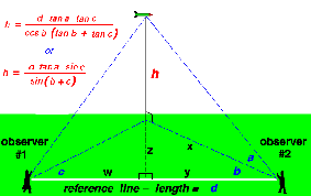
Figure 1 shows a more reliable method of determining altitude. In this method only the distance d, which is the distance between the two observers making the measurements, is required. As shown in the figure only the three angles a, b, and c are required. These angles are the horizontal angles (b and c) between the line connecting the two observers and the line of the rocket’s flight. The other angle (a) is the vertical angle between the ground and the rocket’s location. With this method one observer could measure one angle while the other measures two angles. To make things more robust we will have both observers measure both the horizontal and vertical angles. This will allow us to make two altitude calculations with the same set of data — one set where both angles are used from one observer and the other set where both angles are used from the other observer. Using these measurements the height of the rocket is
 | (14) |
[?]. Beware that this formula assumes that all angles are less than 90 degrees. If your angles are larger, then you have probably made a mistake. When deciding where to locate the observers for your launches, note that this method also gives the best results when the angles are near 45∘ . For this reason, you probably want to set up your observers so that their locations make a equilateral right triangle, with the launching pad at the right angle. In order to get angles near 45∘ for the vertical angles, you will also want the distances from the observers to the launch pad to be roughly the same as the expected maximum altitude of the rocket. Typical apogees for the experiment are roughly 40 m for A engines and 100 m for B engines.
Note that you should end up with four geometrical estimates of the apogee height for each launch — two from the simple one-angle method and two from the multi-angle method.
Note that this semester we will be piloting using an Android tablet app to find the angles.
No matter how you find the angles, be sure to include uncertainty estimates for the angles, and any values that you calculate using the angles.
We will use Mathematica to solve our version of the rocket equation (equation 12). While performing this analysis you can refer to the sample file performing this calculation in a simplified case.
The first step in this calculation is to enter your thrust data. Those groups that determined the thrust curve experimentally should use evaluate their two types of thrust data, and use whichever type they find appropriate here. Be sure to justify your choice. Note that which whichever type of data you use. you need to have your thrust curve defined from 0 up until roughly 5 or 10 seconds. You may want to extend your thrust curve by putting in thrusts of N for times greater than 1 second in your thrust curve files. In other other, add ordered pairs like “1 0” . . . “10 0” to your files.
In order for Mathematica to be able to use this data you must enter the data into a table. To do this you will likely want to use the Import or ReadList function. Something along the lines of
![table1 = Import[“∕home ∕f13∕abstuden∕A8xthrustxdata′′]](rocket_lab13x.png)
![table1=ReadList[“∕home∕f13∕abstuden∕A8xthrustxdata′′,{N umber, N umber, Number, N umber}]](rocket_lab14x.png)
For the A engine data, consider the drag coefficient, cd to be an unknown and solve for it by trial and error for each of the three launches that you did with the A engines. To find cd vary it until your y(t) plot matches your measurements of the rocket flight. Find the mean and standard deviation for the drag coefficient.
For the B engines, use the drag coefficient that you determined above to find a predicted apogee (including uncertainty) for the B engine flights. Also, re-calculate the drag coefficient using your B engine apogee data as the known quantities.
Include a printout of one version of A engine Mathematica analysis and one version of your B engine Mathematica analysis in your lab notebook.
As well as answering the questions listed above, comment on your results.