1 Introduction

Oscillations show up throughout physics. From simple spring systems in mechanics to atomic bonds in quantum physics to bridges blowing the wind, physical systems often act like oscillators when they are displaced from stable equilibria.

In this experiment you will observe the behavior of a simple sort of oscillator: the torsion pendulum. In general a torsion pendulum is an object that has oscillations which are due to rotations about some axis through the object. This apparatus allows for exploring both damped oscillations and forced oscillations.

2 Theory

Note that angular frequency (w in rad/s) and frequency (f in Hz.) are not the same.

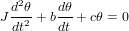
In the damped case, the torque balance for the torsion pendulum yields the differential equation:

(1)

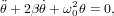
where J is the moment of inertia of the pendulum, b is the damping coefficient, c is the restoring torque constant, and θ is the angle of rotation [“color 2006a]. This equation can be rewritten in the standard form [“color 2004]:

(2)

where the damping constant is β = and the natural frequency is ω₀ = . The general solution to this differential equations is:

(3)

with three different types of solutions possible depending on the relationships between ω₀ and β.

In the underdamped case (β < ω₀):

(4)

with the oscillation frequency ω₁ = , initial amplitude θ₀, and phase γ.

In the critically damped case (β = ω₀):

(5)

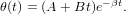
In the overdamped case (β > ω₀):

(6)

where ω₂ = .

For the forced oscillation case, an external torque is added to Equation 1:

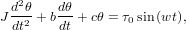(7)

where ω is the driving frequency and τ₀ is the driving torque [“color 2006b]. The general solution to the differential equation is the sum of the homogeneous solutions (which are the solutions to the damped case above) plus a particular solution. The particular solution has the form:

(8)

with

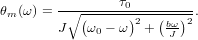(9)

In this case the resonance frequency is ω_r = and the phase shift between the pendulum and the external oscillator is:

(10)

3 Equipment

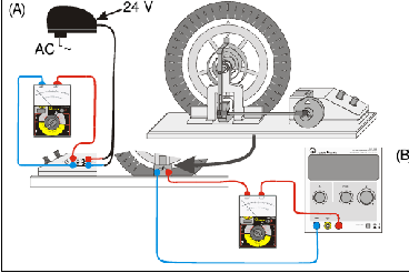
In this experiment you will use the torsion pendulum, the power supply for the driving motor, a low voltage power supply for the eddy current damper, two digital multimeters, and a stop watch.

Figure 1 shows the torsion pendulum and associated electronics. The motor which is used to force the pendulum (which will only be used in the second half of the experiment) is shown on the left of the diagram. The eddy current damping device is shown on the bottom of the diagram.

3.1 Notes on the Torsion Pendulum

• Do not allow the current through the eddy current damper to exceed 2 A.
• Do not leave the current above 1 A for very long.
• The units on for the angle on the pendulum are not standard. Make up a name for the units and stick with it.
• Take the moment of inertia, J, of the torsion pendulum to be 3.0 ± 0.1 kg ⋅ m².
• Do not forget to consider uncertainties in your measurements and calculations.

4 Procedure

4.1 Damped Oscillations

First, setup the torsion pendulum apparatus, with the forcing motor turned off and play with it to get an idea of how it works [“color 2006a].

4.1.1 Nearly Free Motion

With damping magnet turned off, find the natural frequency by measuring the period of the torsion pendulum. You will probably get better results if you use the time it takes the pendulum to oscillate 10 or 20 times to find the period. Note that even with the current off, friction does cause some damping of the pendulum. So the motion is not quite simple harmonic motion.

4.1.2 Damping Constant

Pick a small value of the damping current (0.1 A < I < 0.3 A) and determine the damping constant. To do this first measure the period several times. Then start the pendulum from its furthest rotation point and measure ϕ after each period. If you have difficulty taking the ϕ measurements, you may need to try again.

Plot ϕ versus time. Your plot should follow an exponential envelope. Fit your data to find a value for the damping constant, β.

Repeat this process for a higher value of the damping current (0.3 A < I < 0.6 A).

4.1.3 Nearly Critically and Critically Damped

Increase the damping current until the system only completes one oscillation after you let it go from its furthest rotation point, so the pendulum only crosses 0 once and then approaches 0 from the negative side. Find the oscillation time for this case by taking several measurements and taking the average.

Then increase the current until the pendulum approaches 0 from the positive side, but never crosses 0. This is the critically damped case. Use several measurements for the time it takes the pendulum to reach the equilibrium in this case.

Now use the critically damped case to get an estimate of the damping constant, β, in this case. Find the damping constant from equation 5 by measuring the time that it takes the pendulum to reach some fixed θ, say θ₀ ∕10, after releasing it from its furthest rotation point. Note that in this case you can assume B = 0 and that A = θ(t = 0) in equation 5. Since ω₀ = β in the critically damped case, you can use this β to get estimates of the damping coefficient, b, and the restoring torque, c. Recall that J = 3.0 ± 0.1 kg⋅m².

Now put the current at a higher value (but remember to keep it under 2.0 A). This is an overdamped case. Find the oscillation time in this case.

4.2 Forced Oscillations

First, setup the torsion pendulum apparatus with the forcing motor turned on and play with it to get an idea of how it works [“color 2006b]. Note that you may have to give the pendulum an initial displacement to get it moving, but that initial motion will damp out, leaving only the forced oscillations.

4.2.1 Resonance Curve

Find the resonance frequency of the torsion pendulum from a amplitude versus driving frequency plot for the torsion pendulum.

Set the current through the eddy current brake at an intermediate value (~ 0.4 A). Set the frequency of the driving force by adjusting the applied voltage. Note that you will need to measure the frequency of the driving by timing the period of the driver. The input voltage is not linearly proportional to the frequency. Measure the period of the driver for 10 revolutions and use this measurement to find the period. Measure the amplitude of the oscillation after it has reached a steady state. Note that it may take several minutes for the pendulum to reach a steady state for forced oscillations, especially near the resonance or with small damping. This settling process will likely go more quickly if you stop and restart the pendulum each time that you change the frequency.

Along with the frequency, amplitude, and currents also record the phase shift between the driver and the torsion pendulum. Note that the phase shift can be difficult to determine.

Take enough measurements to get a smooth resonance curve. In particular, be sure to take many measurements near the resonance frequency. Plot these resonance curves, and use them to find the resonance frequency. Use the resonance frequency and the natural frequency found above to find the damping constant for this case.

Repeat this process for a small (I ~ 0 A) and a large (I ~ 0.8 A) damping current.

5 Conclusions

1. Do the damping constants in Section 4.1.2 consistent with with what you would expect? If not, attempt to explain why not.
2. How do the three average oscillation times found in Section 4.1.3 compare? What does this tell you about the critically damped case?
3. In Section 4.2.1, how did the phase difference between driver and the oscillator vary with frequency? What was the phase at low frequency? At high frequency? Near resonance?
4. Are the damping constants found in Section 4.2.1 consistent with those in 4.1.2 ? If not, attempt to explain why not.

References